Modern active sound cancellation is built on a simple physical principle but executed with extremely sophisticated real-time signal science. At the center of the method is destructive interference: when two sound waves of equal amplitude and opposite phase meet, the pressure maxima of one align with the pressure minima of the other, causing the net acoustic pressure to collapse toward zero. This is straightforward textbook acoustics, but modern systems operate in dynamic, unpredictable environments, so the scientific problem is no longer just wave inversion—it is real-time prediction, rapid adaptive filtering, spatial control of sound fields, and compensation for mechanical and environmental delays that would otherwise make cancellation fail. Modern active systems do not simply “play the opposite wave.” They build a continuously updated model of the acoustic field, forecast the next moments of incoming noise, and synthesize an anti-noise signal that reaches the listener at the precise time and position required for cancellation.
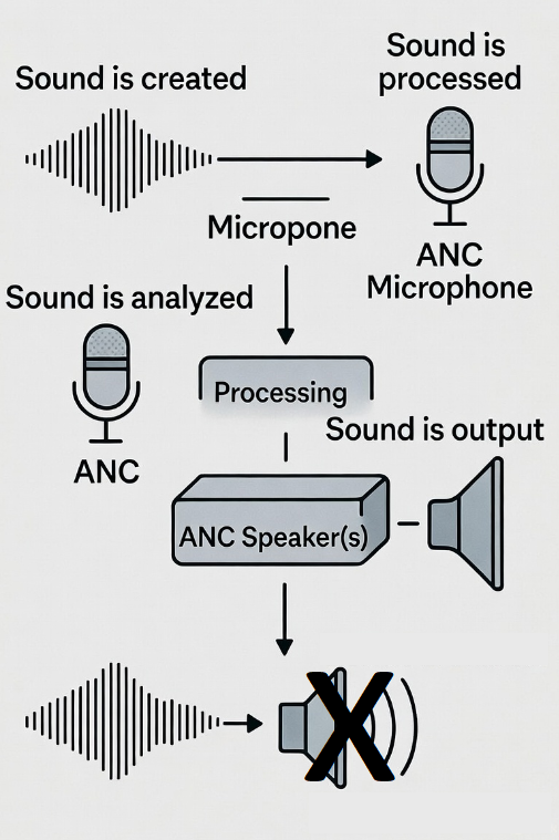
The process starts with sensing. A microphone, or an array of them, captures the incoming noise. These microphones do not function merely as recorders; they are measurement sensors feeding a digital signal processor with a high-resolution stream of pressure fluctuations. Because unwanted noise is rarely steady or predictable, the system must estimate its statistical and spectral characteristics in real time. The signal is decomposed into its frequency components through fast digital transforms or streaming filter banks. From this, the system identifies the dominant frequencies, their harmonics, their temporal evolution, and the directionality of the source. Crucially, the processor must also track the phase of each component, because cancellation requires the anti-noise to reach the listener aligned in time with sub-millisecond precision. The microphone data, therefore, becomes the raw material for a prediction engine that tries to stay ahead of the noise long enough for the speaker to project the inverse waveform at the right moment.
Prediction is necessary because every system has latency. Microphones, analog-to-digital conversion, digital processing, digital-to-analog conversion, amplifier response, and the speaker’s physical diaphragm all introduce delays. Even at microsecond and millisecond scales, these delays would ruin cancellation if the anti-noise signal were generated reactively. Modern systems use adaptive filtering to solve this. The most common strategy is the filtered-x least-mean-square algorithm (FxLMS), a real-time gradient-based method that continuously updates filter coefficients to minimize the residual error between the desired quiet output and the actual sound measured by an error microphone. The “filtered-x” part refers to compensating for the transfer function of the speaker itself—its resonances, distortions, timing delays, and physical placement. The algorithm learns these characteristics over time and includes them directly in the adaptive filter so that the system predicts how the speaker will behave when generating the anti-noise. This allows the algorithm to generate a wave that is not only the inverse of the unwanted noise but also corrected for everything that would otherwise weaken the cancellation.
The speaker is the second half of the system. It produces the anti-noise wave, which is digitally synthesized as the inverse of the predicted noise. The waveform is not simply a flipped copy; it is shaped, filtered, time-shifted, and amplitude-corrected by the adaptive algorithm. The physical speaker must move air to create pressure waves that match the processor’s calculations. Modern designs use lightweight diaphragms with fast transient response so that the anti-noise can be produced with minimal delay. In headphones, the speaker is positioned extremely close to the ear, creating a controlled acoustic chamber where phase relationships can be tightly maintained. In open environments such as rooms, vehicles, or industrial spaces, the challenge is much greater because reflections, turbulence, and complex geometries distort the field. In those cases, multiple speakers and multiple microphones are used to construct a controlled region, and adaptive algorithms extend into full multichannel solutions that attempt to cancel noise at a defined spatial zone rather than a single point.
The real scientific complexity emerges in how these systems maintain stability. Adaptive filters, by nature, adjust their parameters continuously. If the learning rate is too high, the system becomes unstable and oscillates, generating noise rather than canceling it. If the learning rate is too low, the system adapts too slowly and fails to track fast-changing noise. The adaptive controller must strike a narrow balance, and modern implementations use dynamically variable step sizes, frequency-dependent adaptation, and predictive modelling to stabilize the process. In high-end systems, the algorithms maintain multiple parallel predictive filters, each estimating different components of the noise spectrum. Some filters focus on low-frequency steady noise such as engine rumble, while others track mid-frequency transients or speech-like content. The system blends the outputs of these filters to craft a composite anti-noise wave that remains stable even as the acoustic environment changes.
Spatial modeling adds another layer. Sound does not exist as a single waveform in open space; it is a three-dimensional pressure field with interference patterns, reflections, and directional sources. To cancel noise effectively at the listener’s position, the system must understand how sound propagates through the specific geometry of the environment. Some modern systems incorporate real-time room response measurements. Others use embedded acoustic models that estimate transfer functions between noise sources, microphones, and speakers. In advanced applications such as aircraft cabins or industrial enclosures, distributed arrays of sensors track how noise evolves as passengers move, engines change pitch, or airflow patterns shift. The processor updates its spatial model constantly, allowing cancellation zones to remain stable even in non-stationary environments. This is why high-end ANC is now able to create localized quiet regions without requiring a sealed chamber or tightly confined space.
Another important scientific component is the handling of non-linearities. Real environments are not perfectly linear: speakers distort at high amplitudes, microphones saturate, and airflow turbulence introduces chaotic fluctuations that break the simple assumptions of classical acoustic theory. Modern ANC systems incorporate nonlinear adaptive models when needed, using Volterra filters or neural network-enhanced predictors to compensate for distortions that classical linear filters cannot correct. While most ANC remains mathematically linear for simplicity and speed, the presence of nonlinear correction paths allows the system to maintain cancellation when mechanical or environmental effects deviate from ideal behavior.
The final part of the method is residual error minimization. After the anti-noise is produced, a second microphone—placed near the listener or within the cancellation zone—measures the remaining sound. This error microphone feeds its data back to the controller. The entire adaptive filter algorithm uses this error signal as the metric to adjust its coefficients. If the error decreases, the algorithm reinforces the current parameter adjustments. If the error increases, the adjustments are reversed in direction. This closed-loop feedback is what gives modern ANC its ability to adapt continuously and maintain cancellation even when the noise source changes unexpectedly. It is the reason ANC headsets can reduce engine rumble, stabilize against wind bursts, and adapt to shifting cabin acoustics when a user turns their head or changes seat position.
In scientific terms, modern active sound cancellation is a continuous loop of measurement, modeling, prediction, synthesis, and correction. It converts incoming noise into a dynamic acoustic model, predicts its evolution, generates the precise inverse waveform needed to counteract it, and refines the result through real-time feedback. It is fundamentally an applied physics system governed by acoustics, but it is executed through digital signal processing, adaptive control theory, psychoacoustics, mechanical engineering, and computational modeling. The simplicity of destructive interference hides a remarkable amount of scientific engineering behind the scenes, and the result is a technology capable of making certain sound environments dramatically quieter by actively sculpting the pressure field around the listener.
Services:
Voice Control – Vocalize® Sceiver™ – Sound and Voice Therapy